How to Find Similar Images Using Math

Originally published on Medium — June 22, 2020 · 25 min read

Terminology

Before we begin let’s define some terms that we will use throughout the essay:

• Query: A query is a request for data or information from a database or archive.
• Retrieval: The process of getting something back from somewhere.
• Image Retrieval: Any technology that in principle helps to organize digital picture archives by their visual content.

Source Code and Features

All the code used in this blog is publicly available at my GitLab account. Feel free to play around with the code, use your own dataset, and make any modification.

I also made the computed features available for your convenience. The files are quite large (279MB compressed, 569MB uncompressed), so be mindful of any data limitations you may have before downloading. You can download the features using this link.

Opening Remarks

Most of us are probably familiar with search engines such as Google, Bing, DuckDuckGo, and their functionality. You type a series of keywords and expect to get a list of documents with some relationship to the provided tokens. If the system is good, one can expect that the documents at the top of the list will be more relevant than the rest. This paradigm we just described is one of the problems that the field of Information Retrieval tackles every day.

In the previous example, we used plain text as our query. But what if you wanted to look for a particular image? Maybe you liked a particular painting and would like to find similar styles or maybe you are a doctor working with cancer patients trying to find similar images to aid in your prognosis. For both of these cases, the question remains, how do we compare two images? What does it mean for two images to be the same? Well, in the next few sections we will discuss some common methods currently employed to achieve such a goal.

What is an image?

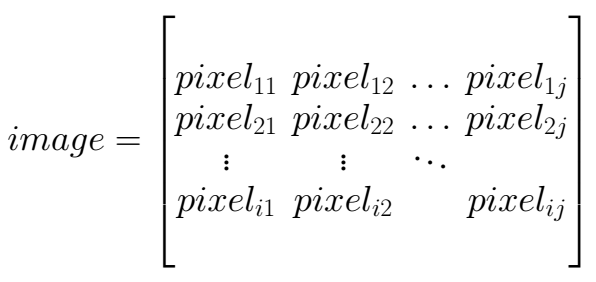
Before moving any further, let’s define how we represent images. In computer vision, we treat images as a matrix of pixels. I don’t want to focus too much on the mathematical definition of a matrix but for the purpose of this essay, you can think of a matrix as a table where items are arranged in rows and columns (see Figure 1) — kind of like an excel sheet.

A pixel is a minute area of illumination that contains three light sources, Red, Green, and Blue (see Figure 2). The number of pixels in a device can be computed from its resolution. For example, most Full High Definition (FHD) 1080p widescreen TVs tend to have a resolution of (1920x1080) which means that there are 1,920 pixels for each row and 1,080 rows in total. If we multiply the number of pixels per row by the number of rows we get a total of 2,073,600 pixels or 2M pixels — keep in mind that this is one example out of many other resolutions and aspect ratios.

Before a device can display a picture it needs to know how bright each pixel needs to be. An image file contains a matrix of pixel values and each pixel value contain three color intensity values (Red, Green, and Blue). This format is known as RGB. The pixel color intensity value ranges from zero (no illumination) to 255 (max illumination). These color values are also called channels. If you pass 255 for every pixel in the red channel and zero for the green and blue channels, all the red lights will be illuminated to the maximum brightness while the green and blue lights will be turned off (see Figure 3). Using this knowledge along with the Additive Color theory, we can generate any color within the RGB color gamut.

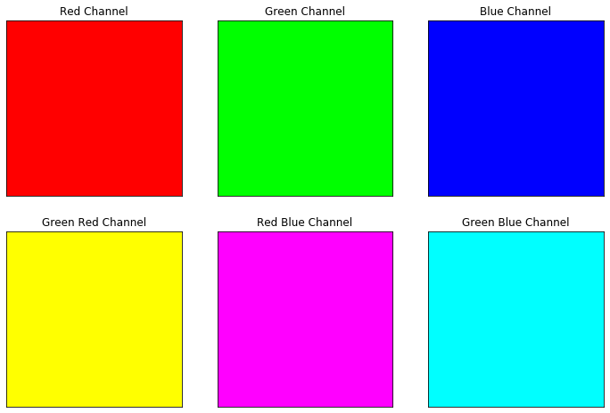
Image Comparison

When we compare an object we need to define a set of characteristics of that object for which to compare against. Let’s take the idiom “comparing apples to oranges” for example. This idiom conveys the idea that the comparison is inefficient since apples have a different set of properties than oranges such as texture, color, size, and flavor profile. The same principle applies to images. Before we can compare two images against each other we need to specify what properties we are comparing.

The three most common image properties that are used for image retrieval are colors, shapes, and textures. In the next few sections, we will discuss both color and shape features as well as the more recently adopted neural features.

Image Retrieval via color

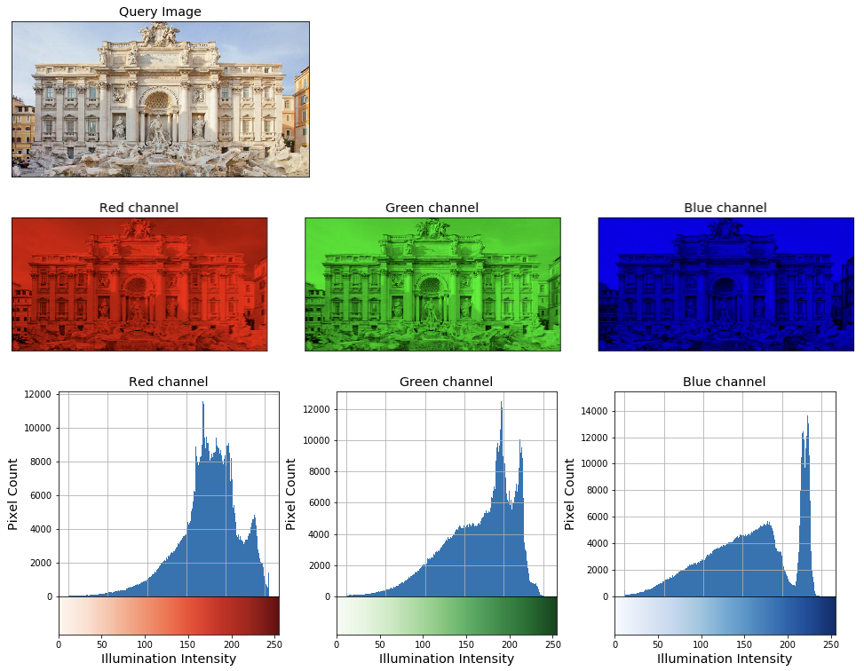
The most simple way to represent an image is by looking at the distribution of colors within the image. Remember that in the previous section we define images as a matrix of pixels where the pixels contained numeric values that represented the illumination intensity of a particular color. We can compute the distribution of color intensities for each channel (Red, Green, and Blue) using a histogram (see Figure 4). All you need to know about histograms is that they aggregate values into bins and count the number of items in each bin.

You might be thinking “why are we computing the distribution of pixels rather than do a 1 to 1 comparison?”. That is a fair question, but remember when we explain the concept of resolution and pixel count? In that example, we had a pixel count of approximately two million. Now imagine we have a database of a thousand equally large images, comparing each pixel in each image against a similar image would require (10⁶ * 10⁶ * 10³) computations or one thousand trillion computations for just one image query. This process would be too slow for any practical application as well as very inaccurate. Because of this, we transform the images into a vector that carries the information in a more compacted way.

Feature extraction Algorithm

1. We begin by separating the image colors into their respective channels.
2. For each channel compute a 48 bin histogram and normalize the output by dividing the bin counts by the total number of pixels.
3. Repeat steps 1 and 2 for every image in the dataset.
4. The result of this computation will be our feature vector for the image.

Fig. 5. Compute the pixel histogram for all images in the dataset and store them as npy files. See the code on GitLab

Similarity metric

Our features should contain three vectors with 48 components. Each vector contains the normalize 48 bin histogram for a particular channel (Red, Green, Blue). As per Chakravarti, et al. [9], we can compute the similarity of two images by the sum of the Euclidean distance of each histogram divided by the number of histograms (see Equation 1).

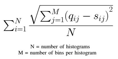
Fig. 6. We define our similarity metric using NumPy arrays and the NumPy linear algebra library. See the code on GitLab

Image retrieval test using color histograms

1. First, we need to load the image features we computed earlier.
2. Select the query features for each class. In this example, I’m picking one query per class to see how the algorithm performs for each class.
3. For every query feature, compute the distance (similarity) for each sample in the dataset and store both the computed distance and the index of the image so we can retrieve it later.
4. For every query feature, sort the dataset images by the computed distance. This will organize images from most similar to less similar.

Fig. 7. Load the color histogram features and define the query set. See the code on GitLab

Fig. 8. Perform Retrieval test and store the Top-5 most similar images for each query image. See the code on GitLab

Results

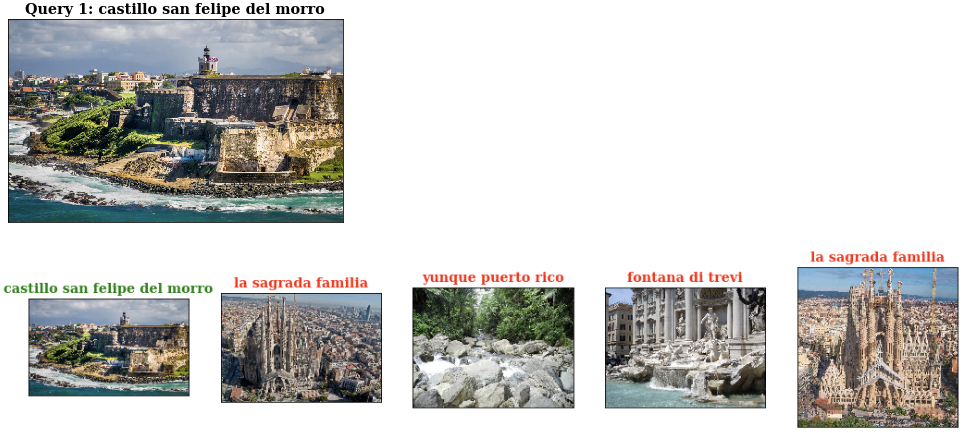
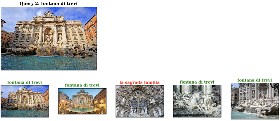
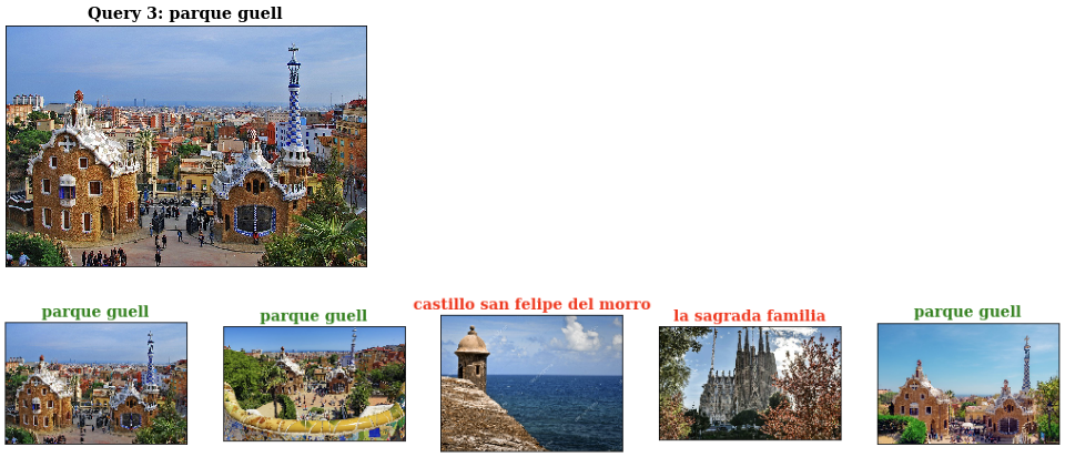
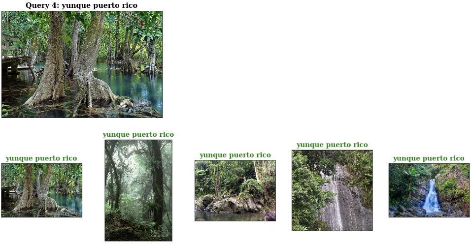
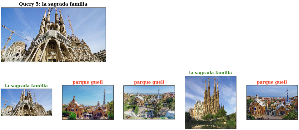
We successfully retrieved a list of images using color histogram features. You might have noticed that most of our queries did not retrieve the proper class of images. This is because the only information we had was a color distribution of all images. On the other hand, we manage to retrieve images that have similar color distributions to our query image (images that are visually similar to our query).

Hopefully, this was an informative introduction to image retrieval via color histogram. There is more exhaustive research on extracting high-quality features based on the color distribution of images that you could expand upon what we saw in this section. If you would like to learn more about image retrieval using color histograms I would recommend reviewing the following papers:

• [9] Chakravarti, R., & Meng, X. (2009, April). A study of color histogram based image retrieval. In 2009 Sixth International Conference on Information Technology: New Generations (pp. 1323–1328). IEEE.
• [10] Han, J., & Ma, K. K. (2002). Fuzzy color histogram and its use in color image retrieval. IEEE transactions on image processing, 11(8), 944–952.
• [8] Kumar, A. R., & Saravanan, D. (2013). Content based image retrieval using color histogram. International journal of computer science and information technologies, 4(2), 242–245.

Image retrieval via shapes

In the previous section, we explored how to retrieve images that contain a similar color distribution. This is good when you are not concerned with the actual content of the images, but what if you wanted to get images that had similar content? For example, you wanted to find images of houses with a similar architecture or even a particular building like the Louvre or the Taj Mahal. This type of image retrieval problem requires more knowledge than just the color distribution. It requires knowledge of the actual shape of the object on the images — for the most part.

Using a technique called convolution we can “scan” an image and filter out contextual information from the images such as edges. If you look at Figure 6, you can see how we can extract horizontal and vertical edges within the image. Using this information we get a better understanding of the spacial qualities of the picture pixels.

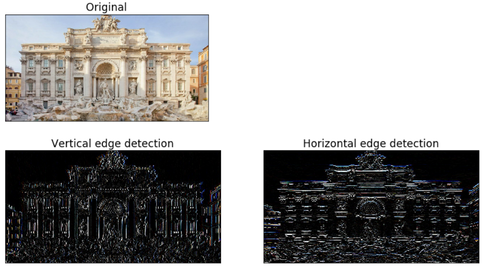
Fig. 11. This is the code that was used to generate the visualization seen in Figure 6. Feel free to try it out with any other image you have around! See the code on GitLab

The use of edge detection for image matching can be traced back to the 1980s where it was leveraged to find locations of interest within an image. Two popular feature extraction algorithms, which are used to this day, are Scale Invariant Feature Transform (SIFT) [3] and Speeded Up Robust Features (SURF) [1].

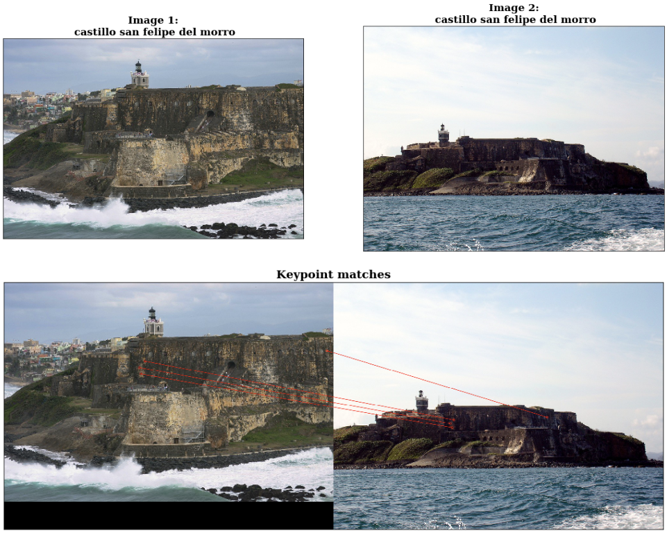
Both of these algorithms are able to find locations of interest — points in the image that standout — within an image. These locations of interest are called keypoints (see Figure 7). For each keypoint in the image, it also computes a feature vector known as a descriptor. Using both the keypoints and descriptors we are able to compare against images that contain similar points of interest even if the objects within the images are at different scales (scale invariance), rotated (rotation invariance), shifted (translation invariance), contain substantial occlusion, and lighting differences.

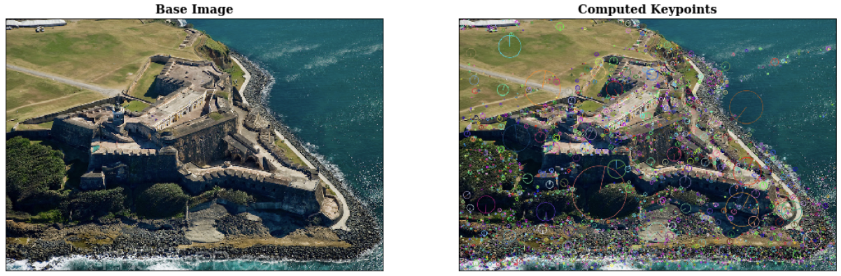
In Figure 8 we can appreciate how similar objects within two distinct images will contain similar keypoints. By extracting the SIFT features of both images we can specify the points of interest shared by instances of the “Castillo San Felipe del Morro”.

Similarity metric

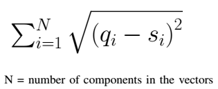
We can use our keypoint descriptors to quantify the similarity of two images. Since our descriptors are just ordinary vectors, we can use any similarity metric that works on vector space. For this test, we will use the euclidean distance also known as the L2-Norm (see Equation 2).

Keypoint matching

Unlike the color histogram features, you cannot just get the closest database descriptors to the query descriptors. As per Lowe, “Many of these initial matches will be incorrect due to ambiguous features or features that arise from background clutter” [3].

Lowe also proposes a method to maximize the likelihood of retrieving correct matches. According to the paper, we can compute the probability that a match is correct by computing the ratio of the distance between the two closes matches.

“The probability that a match is correct can be determined by taking the ratio of distance from the closest neighbor to the distance of the second closest. Using a database of 40,000 keypoints, the solid line shows the PDF of this ratio for correct matches, while the dotted line is for matches that were incorrect.” — Neural Codes for Image Retrieval, Babenco et al.

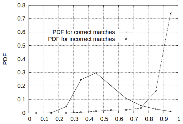
As you can see from Figure 9, the probability of retrieving a correct match increases with the ratio of the distance. We achieve diminishing returns when the distance ratio is higher than 0.70.

Keypoint Correspondence

Once we retrieved a list of good matches, we must make sure that query keypoints and database keypoints belong to the parts of the image for which we are looking for. This is known as a correspondence problem. Random sample consensus (RANSAC) is a popular algorithm used to solve the correspondence problem. Originally proposed by Fischler and Bolles in 1981 [12], RANSAC separates the data into inliers and outliers allowing us to ignore the outliers and only work with the inliers.

Feature extraction Algorithm

• Load the image dataset into memory and define query images for the experiment.

Fig. 15. Load index set and define query images. See the code on GitLab

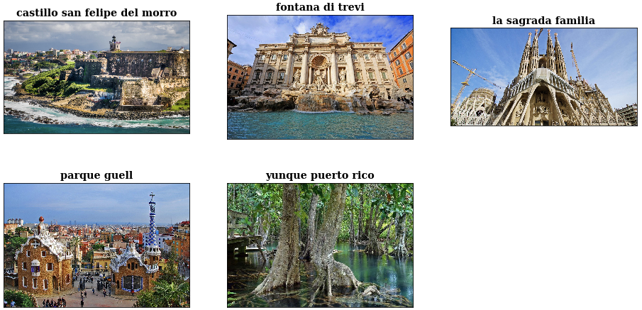
• Extract the SIFT features (keypoints and descriptors) for all the images in both the query and index set.

Fig. 17. Compute SIFT features for all our images. Keep in mind that since we have multiple features for each image, we need a way to map back to the image of origin after performing our similarity computation. This is where the acc_ix (accumulated index) variable comes into play. See the code on GitLab

• Compare every query descriptor against the database descriptors and store the top K nearest keypoints for each class.

Fig. 18. Compute similarity between query images and the index images and store the correct matches as per Lowe’s ratio. See the code on GitLab

• For each descriptor that passes the similarity test, perform geometric verification to make sure we have proper correspondence.

Fig. 19. Perform geometric verification and rank matches by their inlier count. See the code on GitLab

• After performing the geometry verification step, we should have a list of inliers. Select the top K images with the most inliers.

Fig. 20. Perform retrieve and visualize the top-5 ranking results. See the code on GitLab

Results

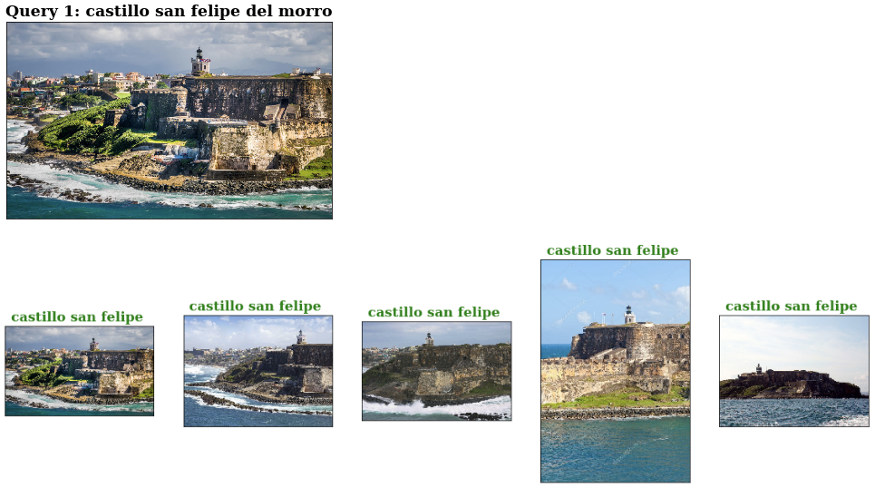
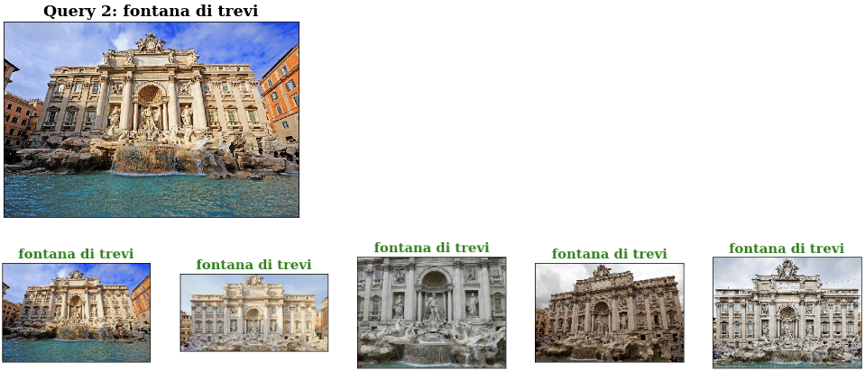
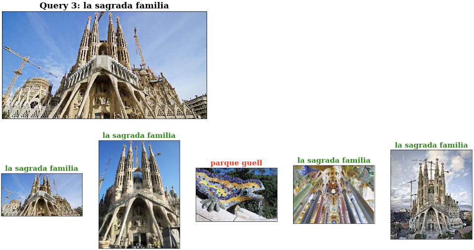
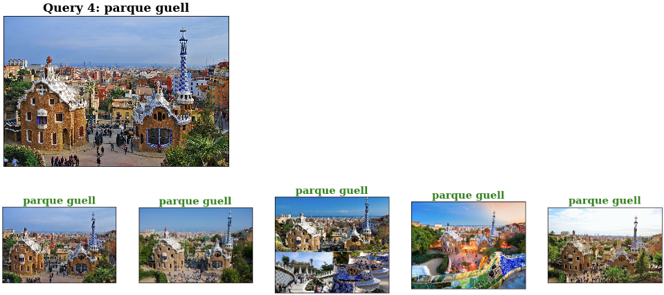
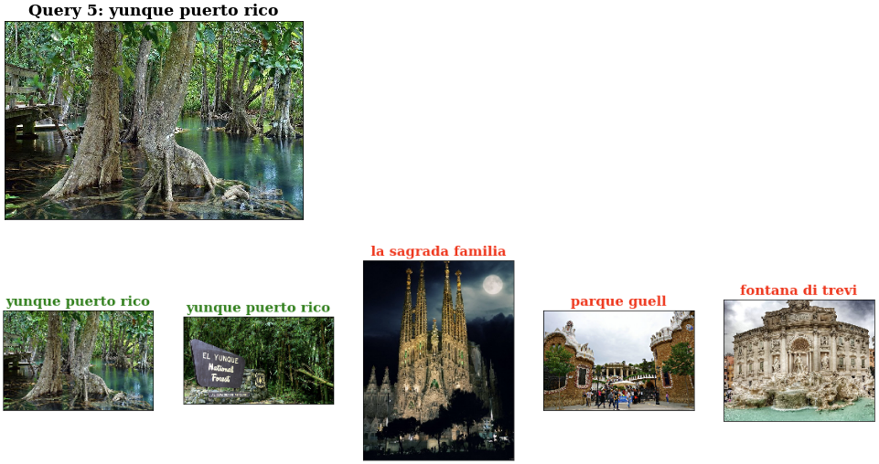
By observing the results, we can see that the retrieval system was able to rank images in our dataset by similarity based on the content of the image. For every query, the first image in the similarity ranking was always the original image. Where this system improves upon the color histogram retrieval system, is in the fact that we were also able to retrieve similar, but distinct, images which share contextual information to our query.

Overall, the retrieval system we created using SIFT features (contextual information) did a better job of retrieving images that contain similar objects to our query images.

Image retrieval using neural networks

In the previous section, we explore how to acquire information regarding the content of an image. We encoded this information into features with the use of the SIFT algorithm. A drawback of such an algorithm is that it lacks overall knowledge about the images it processes. These types of features are called local descriptors. Another drawback of local descriptors is having to compute a large number of features per image, making storage capacity requirement much higher. In our previous example, we had a total of 192 images for which we computed 940,187 features altogether. Even though the images only took 39MB to store, we needed an extra 590MB to store the features. Compare this to the 249KB required to store the Color Histogram features for the same images, and we have a difference of approx. three orders of magnitude higher space complexity.

There is an alternative to local features, called global features. Global features, also known as global descriptors, are features that are calculated over the entire image. A more novel approach to computing global features was proposed by Krizhevsky et al., which claimed that the activation vectors produce by the higher layers in a convolutional neural network (CNN) provided semantical information images that could be computed by their similarity in vector space [15].

“If two images produce feature activation vectors with a small Euclidean separation, we can say that the higher levels of the neural network consider them to be similar.” — ImageNet Classification with Deep Convolutional Neural Networks, Krizhevsky et al.

Later on, this was proven to be true by Babenco et al. [5] when he compared the performance of state of the art image descriptors against the activation of the upper layers of a Convolutional Neural Network.

“It has been shown that the activations invoked by an image within the top layers of a large convolutional neural network provide a high-level descriptor of the visual content of the image. In this paper, we investigate the use of such descriptors (neural codes) within the image retrieval application.” — Neural Codes for Image Retrieval, Babenco et al.

As per Babenco’s findings, the neural features performed competitively when compared to the state of the art features such as the VLAD descriptors. One of the benefits of using CNN to compute our global features is that we can embed properties at training time such as rotational invariance and translation invariance by applying an affine transformation to our images when training the neural network.

Feature Extraction

Within the deep convolutional layers, the network extracts information that will aid in the classification task on the lower fully connected layers. We can observe some of the properties which the convolutional blocks use to better discriminate between classes as seen in Figure 12.

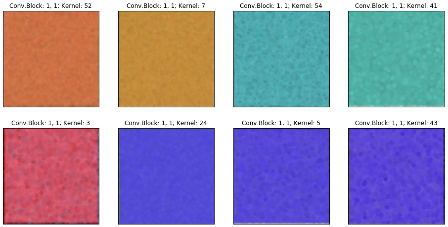
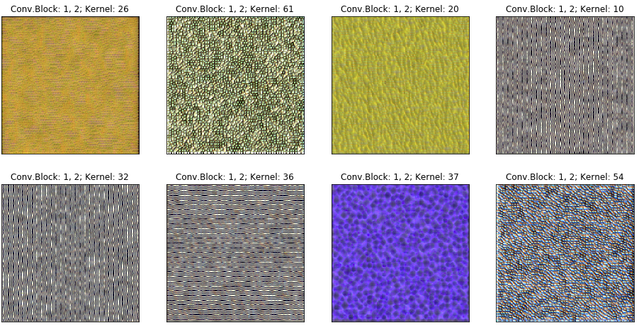
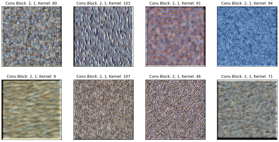
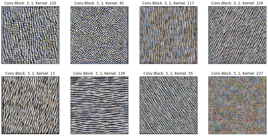
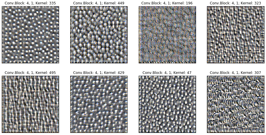
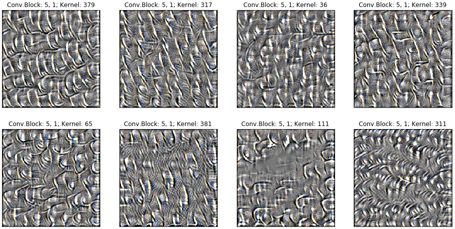
Notice how the initial convolutional layers place higher importance on colors. Moving deeper, we start to see a mix of colors and textures emerge. In the fourth convolutional block, we start to evaluate complex textures and shapes. Finally, in the fifth convolutional layer, we see patterns that look like the creation of an artist.

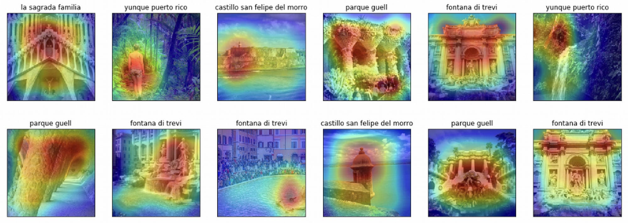
After training a CNN (DenseNet-161) for classification tasks, we are able to compute Convolutional Activation Maps (CAMs) using the gradients. We use this as a mask over our images to see where the networks’ attention lies.

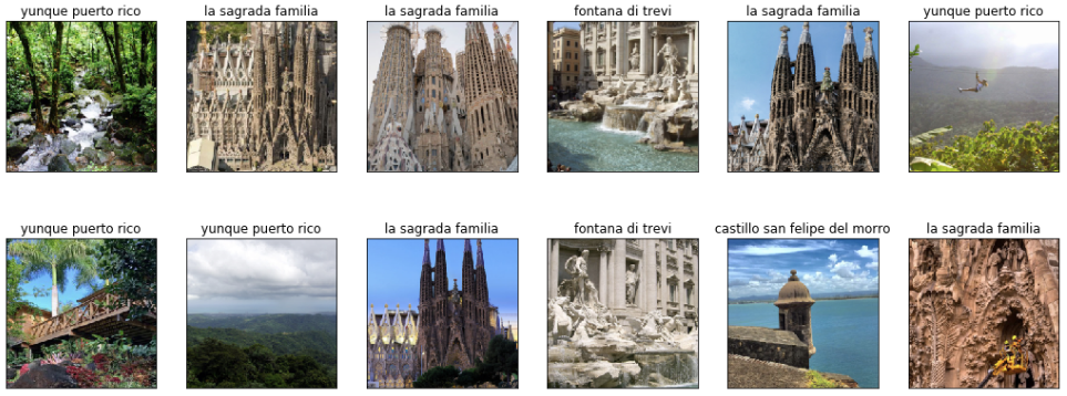
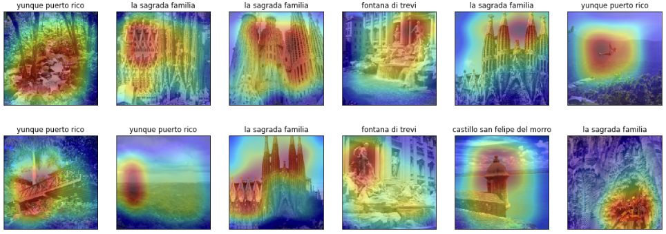
The neural network is able to prioritize locations within the image which provide the most interclass variance. In other words, the euclidean distance between features computed from images of the same class will be smaller than the distance between features computed from distinct classes.

Choosing a CNN architecture

The most important decision when computing deep features — other than your training dataset — is which network architecture to use. There is no clear answer as to which CNN architecture is best for image retrieval. For this test, we kept it simple and downloaded a pre-trained DenseNet-161 from the PyTorch Model Zoo.

Training the network

We used transfer learning to fine-tune a pre-trained DenseNet-161 on our custom 8-class landmark dataset. The idea behind transfer learning is that if we have a model that knows how to perform a task very well, we can take that model and with small modifications, we can have it learn a similar task with very little effort.

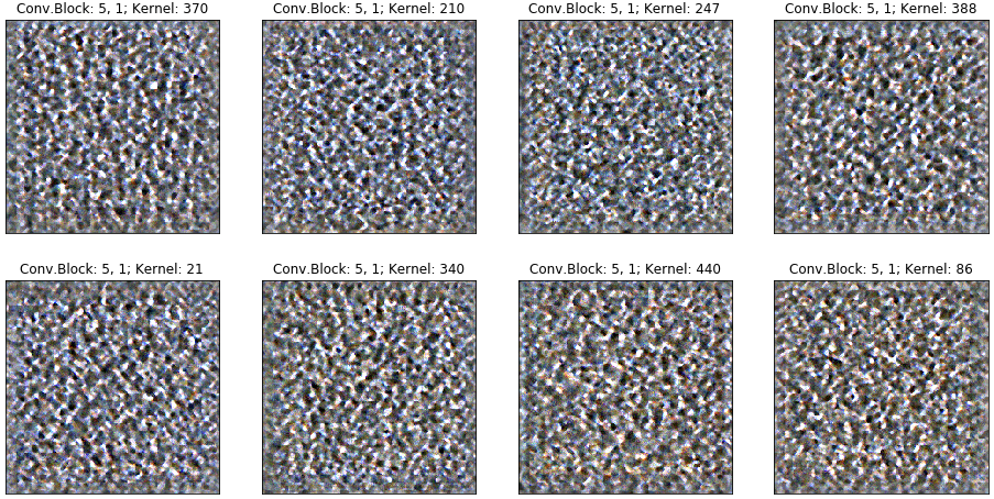
Many of the initial convolution properties are simple enough that they can be learned by most datasets. Once we get to the lower level convolution blocks — block three to five — is where we start to learn representations unique to our images.

Fig. 25. This is the code that was used to download and finetune our model. See the code on GitLab

Similarity Metric

One of the benefits of deep features is that we do not have to worry about correspondence. This means that we can just compute the L2-Norm of the difference between the vectors. The deep features with the smallest euclidean distance will be the most similar.

Algorithm

1. Compute the features for all our index images and store them locally.

Fig. 26. Compute the convolution activation vectors for all our index images. See the code on GitLab

2. Define query set and load features into memory.

Fig. 27. Define query set and load features into memory. See the code on GitLab

3. For every image in our query set, compute the euclidean distance between them and the images in our index ranking them from closest to farthest.

Fig. 28. Preprocessing steps. See the code on GitLab

4. For every query image, visualize the top 5 images in our rank.

Fig. 29. Display the top k images in our query rank. See the code on GitLab

Results

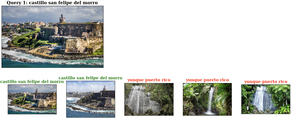
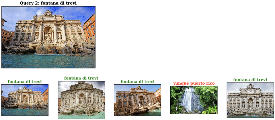
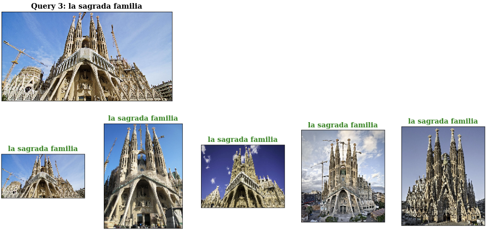
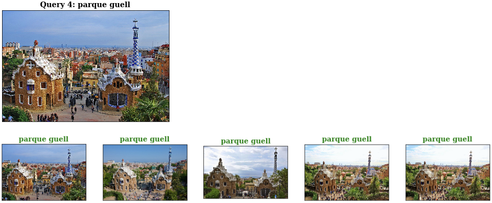
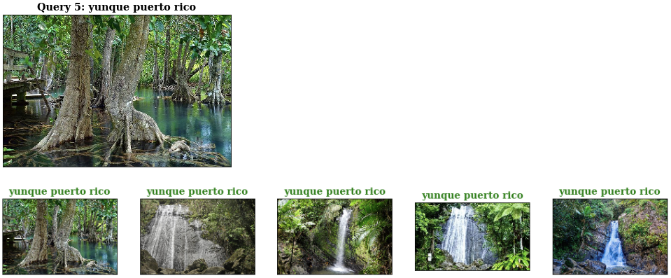
Even though the preprocessing step was a bit more involved, notice how simple it was to retrieve similar images at query time. Overall, the performance of the deep features was comparable to the local descriptors. Storing all of the deep features only took 87MB, this is a substantial reduction in space complexity, with minimal loss in performance, when compared to the SIFT features — this could be further reduced using dimensionality reduction.

Closing Remarks

In this tutorial, we successfully explored some basic algorithms used to this day for image retrieval. We discussed how a simple transformation from pixels to color histograms is decent enough to yield some correct answers. Moving from the simple color distribution, we move to the more complicated and powerful local descriptors. And finally, we concluded our tutorial with a brief example of how machine learning is leveraged to further improve the task of image retrieval.

Keep in mind that you do not have to pick between one or the other. There many other algorithms that mix and match different types of descriptors, creating very rich representations of images. These complex algorithms tend to produce some of the best descriptors, achieving state of the art results, but require a deeper understating of the field.

If you would like to perform your own experiments, feel free to download the codebase available at gitlab.com/nievespg/image_retrieval_blog.

References

• [1] Bay, H., Ess, A., Tuytelaars, T., Gool, L.V.: Surf: Speeded Up Robust Features. Computer Vision and Image Understanding 10, 346–359 (2008)
• [2] Müller, Henning & Michoux, Nicolas & Bandon, David & Geissbuhler, Antoine. (2004). A Review of Content-Based Image Retrieval Systems in Medical Applications
• [3] Lowe, D.G. Distinctive Image Features from Scale-Invariant Keypoints. International Journal of Computer Vision 60, 91–110 (2004)
• [4] Bay H., Tuytelaars T., Van Gool L. (2006) SURF: Speeded Up Robust Features. ECCV 2006.
• [5] Babenko A., Slesarev A., Chigorin A., Lempitsky V. (2014) Neural Codes for Image Retrieval. ECCV 2014.
• [6] B. Zhou, A. Khosla, L. A., A. Oliva, and A. Torralba. Learning Deep Features for Discriminative Localization. CVPR 2016.
• [7] M. D. Zeiler and R. Fergus. Visualizing and understanding convolutional neural networks. ECCV 2014.
• [8] Kumar, A. R., & Saravanan, D. (2013). Content based image retrieval using color histogram.
• [9] Chakravarti, R., & Meng, X. (2009). A study of color histogram based image retrieval. IEEE.
• [10] Han, J., & Ma, K. K. (2002). Fuzzy color histogram and its use in color image retrieval. IEEE Transactions on Image Processing.
• [11] Shafkat, I. (2018). Intuitively Understanding Convolutions for Deep Learning.
• [12] Fischler MA, Bolles RC. Random sample consensus: a paradigm for model fitting with applications to image analysis and automated cartography. 1981.
• [13] Weisstein, Eric W. “Convolution.” MathWorld.
• [14] A. Oliva and A. Torralba. Modeling the shape of the scene: A holistic representation of the spatial envelope. 2001.
• [15] S. A. Chatzichristofis and Y. S. Boutalis. FCTH: Fuzzy Color and Texture Histogram. 2008.
• [16] Krizhevsky, A., Sutskever, I., & Hinton, G. E. (2012). ImageNet classification with deep convolutional neural networks.
• [17] Krizhevsky, A., & Hinton, G. E. (2011). Using very deep autoencoders for content-based image retrieval.
• [18] Simonyan, K., & Zisserman, A. (2014). Very deep convolutional networks for large-scale image recognition.
• [19] Zhou, B., Khosla, A., Lapedriza, A., Oliva, A., & Torralba, A. (2016). Learning deep features for discriminative localization. CVPR.
• [20] Huang, G., Liu, Z., Van Der Maaten, L., & Weinberger, K. Q. (2017). Densely connected convolutional networks. CVPR.